
Track Shares/Stocks with Google Sheets
Use Google sheet to track stocks and indexed funds! Incredibly easy to do, and it is accurate and almost real time. Best of all, you have the data that you can play with to your hearts content. Let’s get started.
Steps
1. Copy Google Sheet
2. Add in Stock Codes
3. Done

Copy the Google Sheet
Easy first step, all you need is to copy my sheet to your drive.
1. Sign up to Google Drive (all you need is a Google account).
2. Go to my workbook (Google Sheet).
3. Go to “File”, and click “make a copy”.

4. Call it whatever you want, and save it wherever you want.

Add in your Share/Stocks/ETF
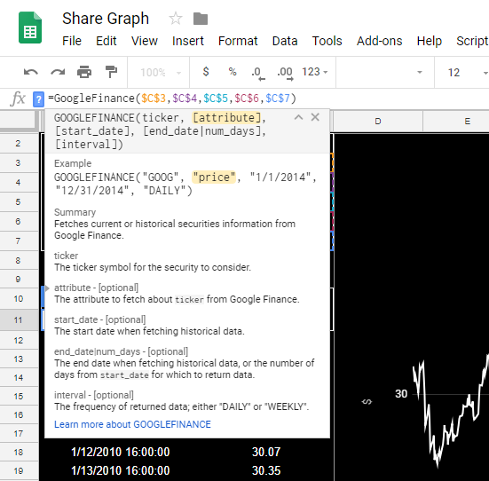
Now all you need to do is use the dashboard! It’s built simply with an IndexMatch formula, and the Google Finance formula. Find out about the Google Finance formula here.
1. Go to “1. Stock Symbols”.
2. All you have to do is find the Exchange and Stock Symbol code to view your data. Take a look at my examples “ExchangeCode:StockCode”.
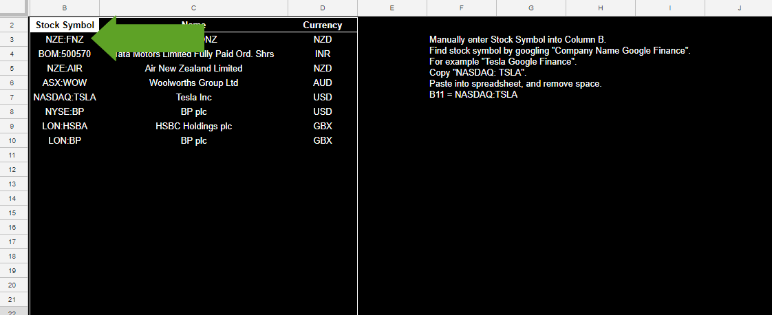
3. To find them, simply Google! Try searching for “Microsoft Google Finance”.
4. In the second line, you can usually see the stock code!

5. Copy it and paste it into anywhere in the B column. “NASDAQ: MSFT” will be copied, however make sure you remove the space after the colon, else the formula won’t work! NASDAQ:MSFT should be copied in.
6. If you did correctly, it will automatically tell you the name of the stock and what currency it is in.

Use the Graph
Now the fun begins, you can look at the graph price for as far back as Google has records!
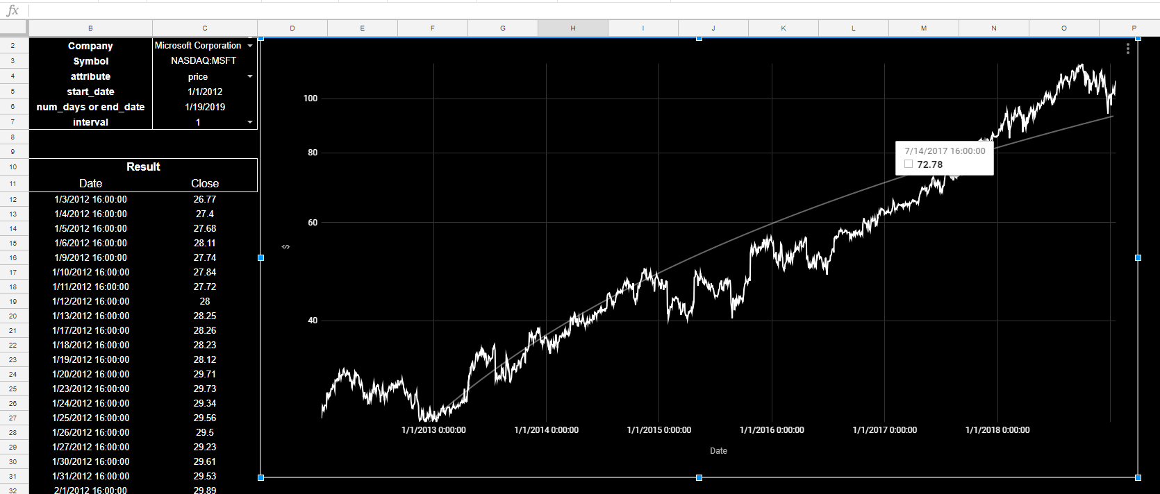
1. Go to the sheet “2. Graph”.
2. In C2, use the drop down box and select a name (this is looking up the C column in the other sheet).
3. Cell C3 then uses an index match to auto populate the Stock Symbol/Code.
4. In cell C4, select “price”. Most of the other options won’t work as it depends on the type of share/stock/etf you are looking at.
5. In C5, select the start date (M,D,Y).
6. In C6, select the end date (M,D,Y).
7. C7 gives you two interval options offered by Google, 1 = Daily, while 7 = Weekly.
8. You would have noticed, that your selections made the data in B/C12 onwards change. This uses an array to push in data depending on your options. Feel free to analyse it to your hearts content!
9. The formula in B11 is the Google Finance function.
10. The graph simply looks at column B and C to row 10,000 (27 Years). Feel free to extend it, export to Excel, or automatically link it using my Google Sheets to Excel tutorial!
11. Now you can look at your investments, and sweat every increase and decrease. For example an ETF I have, while the end of 2018 drop hurt, it just looks like a consistent feature to me! A big drop was overdue.

Just as long as it doesn’t drop too far, and take 8 years to recover…

All done!
Simple as that. There are only two formulas at work here, Google Finance and Index Match. Now all you have to do is modify it and get it working for you!
How about setting up a Google sheet trigger to check if a certain share is above a certain point, and then send you an email alert? This would be an easy task, start by following my Google Sheets Script Scheduling Tutorial.
4. Download
More templates