
Excel’s Personal Macro Workbook - Access your Macros on Any Workbook!
Over the years, I have found and created a bunch of useful small macros. For example, turning off auto formula calculations, unmerging all cells, unhiding all workbooks, adding IFERROR statements to formulas automatically etc.
While great, these would all be unused if I had to copy over the macros to every workbook I worked on. However, you don’t need to do this thanks to the default Excel feature, Personal Macro Workbook!
You save macros to it, and you can use them whenever you want (providing you are on the same computer).
Steps
1. Create Your Personal Macro Workbook
2. Add Macros
3. Create Shortcuts
4. Done
Access your Personal Macro Workbook
For me, it is located here: “C:\Users\Username\AppData\Roaming\Microsoft\Excel\XLSTART\PERSONAL.XLSB”
However, it won’t be there if you never used it before. Plus, there is a much easier way to access it.
1. Open an Excel sheet.
2. Record a macro.
3. Name it anything.
4. Change “Store macro in:” to “Personal Macro Workbook”.
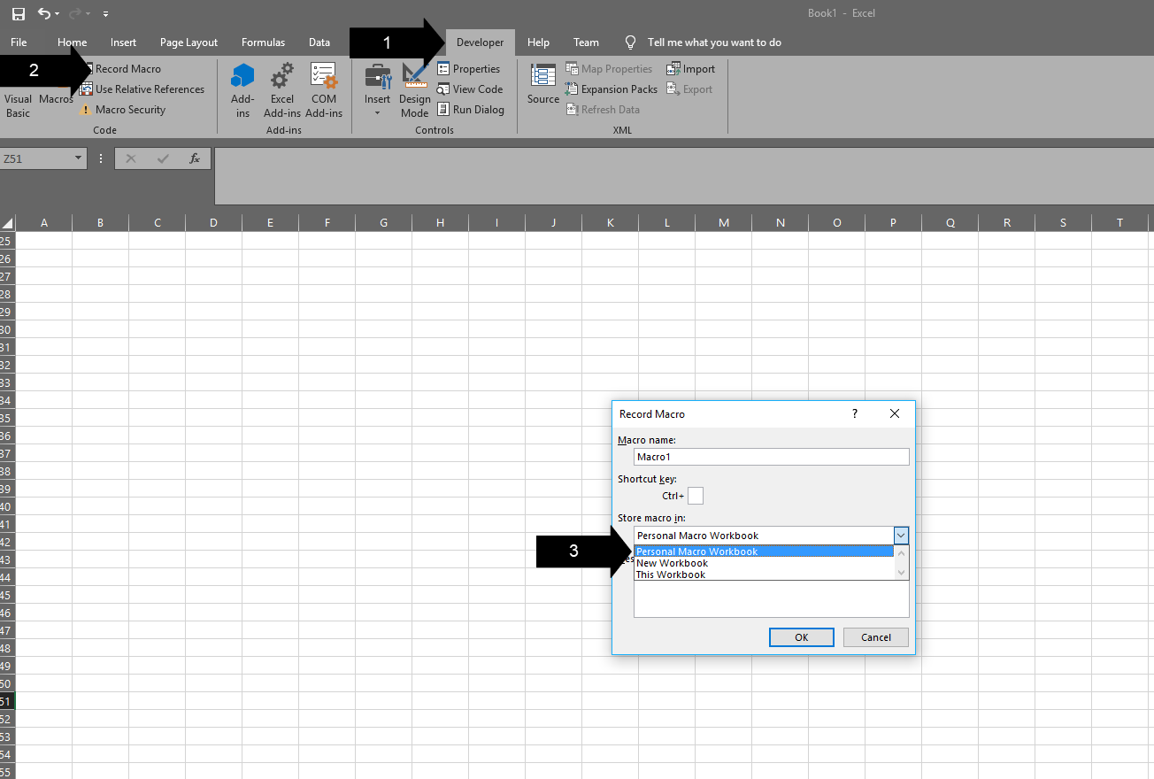
5. Push okay, and write “Excellen” in cell A1.
6. End the recording.
Add your macros
We now have it activated, now you simply add macros to it like any other macro enabled workbook.
1. Open any workbook.
2. Push Alt + F11 or access Visual Basic via the developer pane.
3. You will now see two projects, one for the workbook you have open and another for your personal macro workbook!
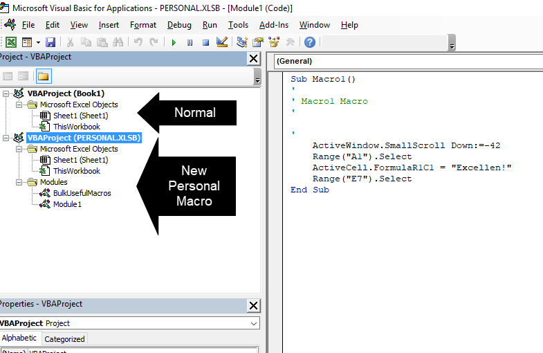
4. This macro will now follow you around wherever you go. Save the VBA editor, and open another workbook to test it out!
Useful Macros to add
You now need some macros to add in, below are some of the useful ones I use. If you download the example workbook below, you can access all of them and copy into your Personal Macro Workbook.
1. Protect Sheet, but only lock formulas! You don’t need to select a range for this one, it works on your active worksheet.
Sub protectFormulasAndEnableProtection()

Dim sht As Worksheet

On Error Resume Next

For Each sht In Sheets
    sht.Activate
    sht.Unprotect
    Cells.Select
    Selection.Locked = False
    Selection.FormulaHidden = False
    Selection.SpecialCells(xlCellTypeFormulas, 23).Select
    If Err.Number = 1004 Then
        'No special cells found (no formulas in this case). Clear the error and take no action
        Err.Clear
    Else
        Selection.Locked = True
        Selection.FormulaHidden = False
    End If
    sht.Protect AllowFormattingColumns:=True, AllowFormattingRows:=True
Next sht

End Sub
2. Remove all hyperlinks. This works on all hyperlinks in the sheet, if you have copied something which has annoying hyperlinks, this is incredibly useful.
Sub RemoveHyperlinks()
   ActiveSheet.Hyperlinks.Delete
End Sub
3. Insert Rows. This opens an input box, and you enter x amount of rows, at a specified rows. Great when you are like me, and constantly screw up your guess on adding x rows to your table!
Sub ToolInsertXRows()
    RowsToInsert = InputBox("How many rows would you like to insert?")
    InsertPoint = InputBox("Which row would you like to insert them at?")

    For Point = 1 To RowsToInsert
        Cells(InsertPoint, 1).Offset(1).EntireRow.Insert
    Next Point
End Sub
4. Save all open workbooks. I often have lots of workbooks open, and when I have to rush off to a meeting, I sometimes just hit the shutdown computer button. This macro saves all open workbooks with one click of the button.
Sub SaveAll()
   Application.ScreenUpdating = False
   Dim Wkb As Workbook
   For Each Wkb In Workbooks
      If Not Wkb.ReadOnly And Windows(Wkb.Name).Visible Then
      Wkb.Save
      End If
   Next
   Application.ScreenUpdating = True
End Sub
5. Change formulas to values. Instead of coping the cell, and pasting as a value – this macro does it with one button click.
Sub FormulasToValues()
Selection.Value = Selection.Value
End Sub
6. Quickly formats data. This is a neat macro, which scrolls to top-left corner, freezes the top row, bolds the top row and Auto Fits the columns.
' Active sheet: Prep for quick viewing
' Scroll to top-left corner, freeze top row, bold top row, AutoFit columns
Sub SetUp_NiceView()

    ' Declare variables
    Dim rowLast         As Long
    Dim colLast         As Integer
    Dim i               As Integer

    ' Maximum column width when AutoFitting columns
    ' Value needs to be in points (you can see the points when clicking-and-dragging to resize a column)
    Const maxColWidth   As Double = 35.86 ' 256 pixels

    ' Set up nice view!
    With ActiveSheet
        ' Unhide all cells
         On Error Resume Next
        .ShowAllData
        .Cells.EntireRow.Hidden = False
        .Cells.EntireColumn.Hidden = False
        On Error GoTo 0

        ' Get last row and column
        ' Excel's Find function remembers the last settings used: Search rows second so the Find function remembers to search by row
        On Error Resume Next
        colLast = .Cells.Find("*", SearchOrder:=xlByColumns, SearchDirection:=xlPrevious).Column
        rowLast = .Cells.Find("*", SearchOrder:=xlByRows, SearchDirection:=xlPrevious).Row
        On Error GoTo 0

        ' If you don't want the code to unhide all cells, use these definitions instead:
        ' colLast = .UsedRange.Columns.Count
        ' rowLast = .UsedRange.Rows.Count

        If rowLast = 0 Or colLast = 0 Then Exit Sub

        ' Bold top row
        .Range(.Cells(1, 1), .Cells(1, colLast)).Font.Bold = True

        ' Freeze top row
        ActiveWindow.FreezePanes = False
        Application.Goto .Cells(2, 1), True
        ActiveWindow.ScrollRow = 1
        ActiveWindow.FreezePanes = True
        .Cells(1, 1).Select

        ' Disable AutoFilter if it's on
        .AutoFilterMode = False

        ' AutoFilter top row
        With .Range(.Cells(1, 1), .Cells(rowLast, colLast))
            .AutoFilter

            ' AutoFit columns
            .Columns.AutoFit

            ' Loop through each column
            ' If any have exceed the max width, try AutoFitting just the header
            ' If the column still exceeds the max width, set it to the max width
            For i = 1 To colLast
                If .Columns(i).ColumnWidth > maxColWidth Then
                    .Columns(i).Cells(1).Columns.AutoFit

                    If .Columns(i).ColumnWidth > maxColWidth Then
                        .Columns(i).ColumnWidth = maxColWidth
                    End If
                End If
            Next i
        End With
    End With

End Sub
7. Turn off the page break lines. This is almost my favourite, as I constantly accidentally turn on the Page Layout view. This adds in lines, which you can only get rid of by going into the Excel settings. Now it is a button click!
Sub HidePageBreaks_Toggle()

    ActiveSheet.DisplayPageBreaks = Not ActiveSheet.DisplayPageBreaks

End Sub
8. Unhides all Sheets. I use this the most, simple and effective.
' Active workbook: Unhide all sheets
Private Sub Unhide_AllWorksheets()

    ' Declare variables
    Dim currentScreenUpdating   As Boolean
    Dim ws                      As Worksheet

    ' Set up
    currentScreenUpdating = Application.ScreenUpdating
    Application.ScreenUpdating = False

    ' Unhide the sheets
    For Each ws In ActiveWorkbook.Worksheets
        ws.Visible = xlSheetVisible
    Next ws

    ' Clean up
    ActiveWindow.Activate
    Application.ScreenUpdating = currentScreenUpdating

End Sub
9. Change Formula Calculation to Manual. This is a must for large datasets.
Sub CalcManual()
Application.Calculation = xlCalculationManual
Application.StatusBar = "WARNING: Calculation has been set to manual"
End Sub
10. Change Formula Calculation to Automatic. Saves going to the settings page!
Sub CalcAuto()
Application.Calculation = xlCalculationAutomatic
Calculate
Application.StatusBar = False
End Sub
11. Filter Selected Values. If you have a table, you click on the cell and run the macro. It filters the table by the contents of that cell.
Sub FilterSelectedValues()
    Dim arrayEn() As Variant
    Dim selCol As Integer
    Dim rCell As Range
    Dim i As Long

    ReDim arrayEn(1 To 1, 1 To Selection.Count)
    selCol = Selection.Column
    i = 1

    For Each rCell In Selection
       arrayEn(1, i) = CStr(rCell.Value2)
       i = i + 1
    Next rCell

    ActiveSheet.Range("A1").AutoFilter Field:=selCol, Criteria1:=arrayEn, Operator:=xlFilterValues
End Sub
12. Unhide rows and columns. Saves you having to do ctrl + a and unhiding!
'This code will unhide all the rows and columns in the Worksheet
Sub UnhideRowsColumns()
Columns.EntireColumn.Hidden = False
Rows.EntireRow.Hidden = False
End Sub
13. Unmerge all cells. Blasted merged cells. Please, please use Centre across Selection instead.
'This code will unmerge all the merged cells
Sub UnmergeAllCells()
ActiveSheet.Cells.UnMerge
End Sub
14. Centre Across Selection. Speaking of, this is a better way to merge cells. It doesn’t actually merge them, only visually. Else you need to go into the Alignment settings tab to access this.
Sub CenterAcrossSelection()
    Selection.HorizontalAlignment = xlCenterAcrossSelection
End Sub
15. Highlight Alternate Rows. If you ever want to highlight every second row in a table, this is for you. Select your data, and run the macro. Feel free to edit the colour.
'This code would highlight alternate rows in the selection
Sub HighlightAlternateRows()
Dim myRange As Range
Dim Myrow As Range
Set myRange = Selection
For Each Myrow In myRange.Rows
   If Myrow.Row Mod 2 = 1 Then
      Myrow.Interior.Color = vbCyan
   End If
Next Myrow
End Sub
16. Highlights Cells with Spelling Errors. This works in the active sheet – and avoids you having to use the annoying spell check.
'This code will highlight the cells that have misspelled words
Sub HighlightMisspelledCells()
Dim cl As Range
For Each cl In ActiveSheet.UsedRange
If Not Application.CheckSpelling(word:=cl.Text) Then
cl.Interior.Color = vbRed
End If
Next cl
End Sub
17. Highlight Blank Cells. You select a range, run the macro and it will highlight the blanks.
'This code will highlight all the blank cells in the dataset
Sub HighlightBlankCells()
Dim Dataset As Range
Set Dataset = Selection
Dataset.SpecialCells(xlCellTypeBlanks).Interior.Color = vbRed
End Sub
18. Auto Fit Columns. This saves you having to double click!
Sub AutoFitColumns()
Cells.Select
Cells.EntireColumn.AutoFit
End Sub
19. Auto Fit Rows. This also saves you the double click, I usually end up merging Auto Fit Columns and Auto Fit Rows together.
Sub AutoFitRows()
Cells.Select
Cells.EntireRow.AutoFit
End Sub
20. Highlight Duplicate Values. This is easier than conditional formatting – highlight your range and it highlights the duplicates values!
Sub HighlightDuplicateValues()
Dim myRange As Range
Dim myCell As Range
Set myRange = Selection
For Each myCell In myRange
If WorksheetFunction.CountIf(myRange, myCell.Value) > 1 Then
myCell.Interior.ColorIndex = 36
End If
Next myCell
End Sub
21. Insert Multiple Sheets. You enter in how many sheets you want, and it creates them for you!
Sub InsertMultipleSheets()
Dim i As Integer
i = InputBox("Enter number of sheets to insert.", "Enter Multiple Sheets")
Sheets.Add After:=ActiveSheet, Count:=i
End Sub
22. Resize all Charts in Sheet. I use this a lot. It resizes all charts to 300 by 200. Depending all your requirements, modifier the macro to generate an Input box so you can input your exact size!
Sub Resize_Charts()
Dim i As Integer
For i = 1 To ActiveSheet.ChartObjects.Count
With ActiveSheet.ChartObjects(i)
.Width = 300
.Height = 200
End With
Next i
End Sub
23. Table of Contents. This could be useful depending on your work. If you have a ton of sheets in a workbook, this macro creates a new sheet with a Hyperlink to each sheet.
Sub TableofContent()
Dim i As Long
On Error Resume Next
Application.DisplayAlerts = False
Worksheets("Table of Content").Delete
Application.DisplayAlerts = True
On Error GoTo 0
ThisWorkbook.Sheets.Add Before:=ThisWorkbook.Worksheets(1)
ActiveSheet.Name = "Table of Content"
For i = 1 To Sheets.Count
With ActiveSheet
.Hyperlinks.Add _
Anchor:=ActiveSheet.Cells(i, 1), _
Address:="", _
SubAddress:="'" & Sheets(i).Name & "'!A1", _
ScreenTip:=Sheets(i).Name, _
TextToDisplay:=Sheets(i).Name
End With
Next i
End Sub
24. Paste as Picture. You select a range, and this creates a picture copy.
Sub PasteAsPicture()
Application.CutCopyMode = False
Selection.Copy
ActiveSheet.Pictures.Paste.Select
End Sub
25. Changes Zero to Blank. This macro is a formula (similar to my split out number and text macro). ZeroToBlank(x). Gets rid of the long If(x=0,”“,x).
Public Function ZeroToBlank(x As Integer) As String
    If x = 0 Then
        ZeroToBlank = ""
    Else
        ZeroToBlank = CStr(x)
    End If
End Function
26. Remove Decimals. Simple but useful, removes the decimals from your selection.
Sub removeDecimals()
Dim lnumber As Double
Dim lResult As Long
Dim rng As Range
For Each rng In Selection
rng.Value = Int(rng)
rng.NumberFormat = "0"
Next rng
End Sub
27. Wrap Formulas in IFERROR. Made a bunch of formulas, but forgot about IFERROR? Simply select them, run the macro, and input what you want returned!
Sub IFERRORconvert()

'This macro places the entire function in each cell of a selection inside of an IFERROR function.
'The user may enter the desired argument for value if error, as a string or a number.

Dim errorString As String
Dim resultString As String

errorString = Application.InputBox("Enter the value to return " & Chr(10) & "if an error condition is found:", "Enter error condition return value:", "0")

Application.Calculation = xlCalculationManual

For Each c In Selection
    resultString = "=IFERROR(" + Right(c.Formula, Len(c.Formula) - 1) + "," + errorString + ")"
    c.Formula = resultString
Next

Application.Calculation = xlCalculationAutomatic

End Sub
28. Wrap Formulas in IF Statement. I modified the above IFERROR code to wrap the formula in If Statement. For example if Sum(A1,A2) = 0, and you want it to return ““, this macro makes this easy to do!
Sub IFconvert()

'This macro places the entire function in each cell of a selection inside of an IF function.


Dim errorString As String
Dim errorString2 As String
Dim resultString As String

errorString = Application.InputBox("IF = to what? " & Chr(10) & "Recommend 0 or """"", "Enter what to equal:", "0")
errorString2 = Application.InputBox("Enter the value to return ", "Enter condition return value:", """""")

Application.Calculation = xlCalculationManual

For Each c In Selection
    resultString = "=IF(" + Right(c.Formula, Len(c.Formula) - 1) + "=" + errorString + "," + errorString2 + "," + Right(c.Formula, Len(c.Formula) - 1) + ")"
    c.Formula = resultString
Next

Application.Calculation = xlCalculationAutomatic

End Sub
How to get use out of the macros
If you add all of them, chances are you won’t use them if you need to go to the developer tab and click the macro button. Try some out, and create keyboard shortcuts and add them to the quick access toolbar.
1. Click on the Macro button in developer pane.
2. Make sure “Macros in:” says “Personal.xlsb”.
3. Click on a Macro and click on “Options”.
4. Add in your shortcut.
5. Click “OK”!

And/or:
1. At the top left corner of your screen, click on the drop down arrow on the Quick Access Toolbar.
2. Click on “More Commands”.

3. Change “Popular Commands” to “Macros”.
4. Click on one of your macros.
5. Click the “Add > >” button.
6. Click “OK”.

7. You now have your macros on the Quick Access Toolbar!

That’s it, you can now customize Excel to you!
Start recording your own macros, and make Excel work for you. Why not write a macro that formats a table exactly how you want it? And add it your quick access bar?
If you want another cool macro to add, try the Split Numbers from Text Tutorial.
Download below to get a workbook with all the above macros.
7. Download
More templates