
Index Match Match Function - Ultimate Vlookup and Index Match!
/Index Match Match
This great formula lets you search the x and y axis to lookup an item. In my opinion, this is currently the most quintessential Excel formula.
Our task today will be to create a simple dashboard, which looks up a tiny data table.
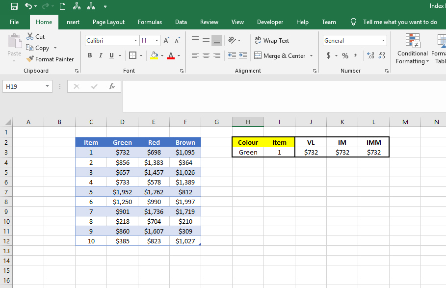
H3 and I3 have data validation, where the user can select the item and color.

We now need a formula that can look up the data table based on the users choice.
Vlookup
Vlookup is probably the most popular formula used by inexperienced Excel users. Which is most of the population. It does certain jobs well, but is mostly redundant once you learn Index Match. Utterly unneeded when you learn Index Match Match.
For example, when writing this tutorial it took me a couple of minutes to remember how to use Vlookups! As I now never use them!
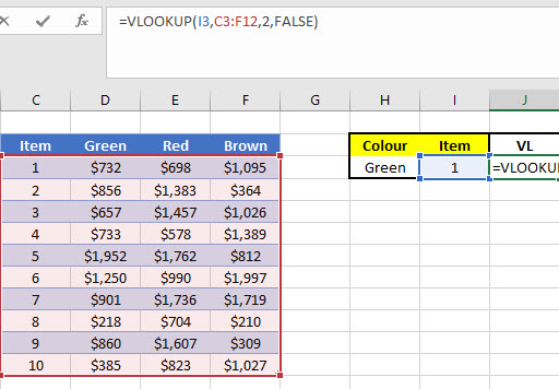
To remind you about Vlookups,
VLOOKUP(item in column to lookup, range of data - item to lookup must be in first column, column number in range to return, FALSE means it will only accept an exact match)
So we can get a lookup for the item, but what about for the color?
Due to the formula accepting a column number, you can get Vlookups to do what we want with a little bit of extra work. Create three hidden helper columns, create a table where the color is assigned to a column number, Hlookup based on H3 and make your Vlookup reference the Hlookup result. Clear as mud?
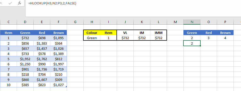

So although we needed 3 helper columns, plus another formula, it can work!

This was the only reason I used Vlookups after discovering Index Match.
Index Match
Index Match is better than Vlookups. I have written about this before, but essentially it is more resource efficient and harder to break.

INDEX(column range you want returned,MATCH(Lookup Item, Column Range of lookup items, 0 for exact match))
It is more resource efficient as it is only looking at a couple of columns, not the entire range. It is more robust as it uses actual column references, not a static column number. So if you insert a new column in the middle of your data table, it won’t break the formula!
However, this doesn’t allow you to search the x axis to find the color. You could remove the absolute ($) reference from column D and then drag it over to change your dashboard slightly. Or you could do something similar to the Vlookup example above, however you would use INDIRECT formulas to change the column letters. Instead of mucking around with that, add in a second MATCH!
Index Match Match
Index Match Match makes this easy. No helper columns, no mucking around. It is more resource intensive than Index Match, no more than Vlookup.
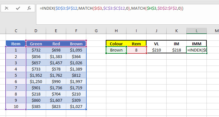
Looks complex, but range of data, Y axis match first, X axis match second.
INDEX(Range of data - do not include the lookup columns/rows!, MATCH(Y axis lookup, Y axis column range, 0 for exact match), MATCH(x axis lookup, x axis row range, 0 for exact match))
Another great thing is that the lookup cells don’t need to be anywhere near the data range.
Notice how the Vlookup is broken, but Index Match Match (and Index Match) still works fine.
So there you have it. Index Match Match.
As I write this, there is talk about something called Xlookup coming out. From what I understand this is still less relevant than Index Match Match, but time will tell!
You now have an easier formula, but how about an even easier life? Learn how to automate Excel tasks with my Schedule Excel Macro Tutorial. If you want to automate other tasks, take a look at my PowerShell Macro Tutorial!